Browsing a curated database¶

A common source of problems for new users of AiiDA often arises when they receive an exported database and want to get an idea of its content but don’t know how.

In the following section we will use the database from “Two-dimensional materials from high-throughput computational exfoliation of experimentally known compounds”.

The final goal will be to create a table of the value of the band gap for a set of 2D materials from this study, filtering only those where the band gap is below a given value.

We will show you here, step by step, how to start from a new unknown database, understand its layout, and eventually prepare the final query. This will give you some guidance on how to apply and extend queries for your own needs.

This story can be run in the Quantum Mobile 20.03.0 virtual machine, that you need to download and install first (unless you have AiiDA already installed on your computer; we are using AiiDA 1.3 here). You will also need to download and import the 2D materials database from the corresponding Materials Cloud Archive entry This can be easily done by running the following commands in your AiiDA environment:

(aiida) max@qmobile:~$ wget 'https://archive.materialscloud.org/record/file?file_id=d1f3ac29-e3b0-400b-8109-8455be66160b&filename=two_dimensional_database.aiida&record_id=18' -O 2D_database.aiida
(aiida) max@qmobile:~$ verdi import 2D_database.aiida

Using the discover section¶

In the case of this particular database, an interface that allows easy exploration of curated results is available through the corresponding Discover section of Materials Cloud. This interface will provide a general overview of all materials available, and choosing any of them (let’s say, silver bromide) will give you access to its available calculated properties, as well to information on the provenance of such properties.

In this story, we are interested in the band gap of a material. You can then use the Explore button (the little AiiDA icon) next to the text Band gap [eV]: 1.3 to go to the actual node that contains this value. Similarly, you can click on the Explore button next to the band structure plot to inspect the BandsData node, and so on. We invite you to browse the Discover and Explore sections for this database on you own, to get an idea of the features offered by the Materials Cloud interface.

For our purposes, now we will just take note of the UUID of the Dict node containing the value of the band gap (89315c33-2f9b-41ab-b7d4-22aff0ae75f4) and we will see together how to check all information in the local database that you have imported earlier.

Manually browsing the database¶

Now that we have a local instance of this database, we can see how to get some information regarding our node of interest (identified previously as the one that contains the band gap energy of AgBr). For this we will use the AiiDA interactive shell:

(aiida) max@qmobile:~$ verdi shell

We start by performing some browsing using the AiiDA API to explore the properties and connections of this node.

Load the node by using its UUID (note that the integer identifiers, called PKs, will most probably be different in your DB, but the UUIDs will always be the same):

In [1]: bandgap_node = load_node('89315c33-2f9b-41ab-b7d4-22aff0ae75f4')
In [2]: bandgap_node
Out[2]: <Dict: uuid: 89315c33-2f9b-41ab-b7d4-22aff0ae75f4 (pk: 4625)>

One can check the attributes and discover that the band gap is in eV and is stored in the attribute named band_gap (knowing that the parser always returns eV, we are not going to use the units in the following, but one could generalise the query later if necessary).

In [3]: bandgap_node.attributes
Out[3]: {'band_gap': 1.25790023795923, 'band_gap_units': 'eV', 'is_insulator': True}

We start inspecting the provenance using the .creator method to get the calculation that generated the Dict data node:

In [4]: calculation_node = bandgap_node.creator
In [5]: calculation_node
Out[5]: <CalcFunctionNode: uuid: 43b7e596-130c-4733-b3dd-13b264b845a0 (pk: 3028)>

Then we can use .inputs.LABEL_NAME to access any of the inputs of this calculation. In our case, we will be interested in the one labeled bands (note that you can use tab completion to discover all input link labels: after .inputs. press the TAB key twice to see all available labels):

In [6]: bands_node = calculation_node.inputs.bands
In [7]: bands_node
Out[7]: <BandsData: uuid: 7fbb633d-a224-46b7-84b1-74a3ceca81e0 (pk: 4689)>

In the same way we did before, we can now check the calculation that created this BandsData node (i.e., the band structure), to discover that it was a Quantum ESPRESSO run:

In [8]: qecalc_node = bands_node.creator
In [9]: qecalc_node
Out[9]: <CalcJobNode: uuid: 2a304b31-5a60-4884-bfe7-3c0b1d2c67fc (pk: 57863) (aiida.calculations:quantumespresso.pw)>

Finally, we can check another input one level up to find the original crystal structure:

In [10]: qecalc_node.inputs.structure
Out[10]: <StructureData: uuid: ba8bbdd9-defc-4292-af7d-ed3eb73f778e (pk: 53436)>

Note that we don’t really need all of the intermediate node variables. We did it mostly for convenience, but all of these steps can just be concatenated in a single long chain, as follows:

In [11]: bandgap_node.creator.inputs.bands.creator.inputs.structure
Out[11]: <StructureData: uuid: ba8bbdd9-defc-4292-af7d-ed3eb73f778e (pk: 53436)>

The advantage of the long string above is that after every dot you can use tab completion, and therefore (once you get used to it) it becomes very quick to browse advanced provenance graphs in the verdi shell.

One more thing one might want to do is to check if there is a better way to distinguish the CalcFunctionNode that I got at Out[5] above (stored in calculation_node = bandgap_node.creator). Let us check its attributes:

In [12]: bandgap_node.creator.attributes.keys()
Out[12]: dict_keys(['function_name', 'sealed', 'first_line_source_code', 'namespace', 'source_code', 'source_file'])
In [13]: bandgap_node.creator.attributes['function_name']
Out[13]: 'get_bandgap_inline'

This information will be useful in the following section, and will basically allow us to perform a query by filtering by the original function name.

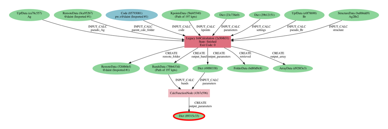
Now, after all these steps, we have a better understanding of the the structure of the data. Another useful tool to get a good idea of the connectivity is the graph generator. One can use verdi node graph generate to visualize the provenance surrounding a node. Limiting it to four levels up (ancestors) will be enough for this case; we will also avoid to show any descendants, since we are not interested here in calculations that used the data node as an input. Note that this command has to be executed outside of the verdi shell.

(aiida) max@qmobile:~$ verdi node graph generate --process-in --process-out --ancestor-depth=4 --descendant-depth=0 89315c33

The result should look something like this:

provenance

Systematic querying of the database¶

Now that we have understood broadly the data layout (provenance links between nodes, their types, and some of the relevant attributes keys and values), let’s now construct a query using the QueryBuilder in order to get the band structure of a set of 2D materials. Create a new text file and copy the content below (these are essentially python scripts, so you can use the .py extension). There are some comments which explain the purpose of each line of code, please read them carefully to understand how the query is constructed. If you are not familiar with the QueryBuilder, we refer to the official AiiDA documentation for more details <https://aiida.readthedocs.io/projects/aiida-core/en/v1.3.0/howto/data.html#finding-and-querying-for-data>_.

from aiida.orm import QueryBuilder, Dict, CalculationNode, BandsData, StructureData

# Create a new query builder object
query = QueryBuilder()

# I want, in the end, the 'band_gap' property returned ("projected")
# This is in the attributes of the Dict node
# As an additional challenge, I also want to filter them and get only those where the band gap (in eV) is < 0.5
query.append(
    Dict,
    project=['attributes.band_gap'],
    filters={'attributes.band_gap': {'<': 0.5}},
    tag='bandgap_node'
)

# This node must have been generated by a CalcFunctionNode (so, with outgoing link the node of the previously
# part, that we tagged as `bandgap_node`, and I only want those where the
# function name stored in the attributes is 'get_bandgap_inline'
query.append(
    CalcFunctionNode, 
    filters={'attributes.function_name': 'get_bandgap_inline'},
    with_outgoing='bandgap_node',
    tag='bandgap_calc'
)

# One of the inputs should be a BandsData (band structure node in AiiDA)
query.append(BandsData, with_outgoing='bandgap_calc', tag='band_structure')

# This should have been computed by a calculation (we know it's always Quantum ESPRESSO
# in this specific DB, so I don't add more specific filters, but I could if I wanted to)
query.append(CalculationNode, with_outgoing='band_structure', tag='qe')

# I want to get back the input crystal structure, and I want to get back
# the whole AiiDA node (indicated with '*') rather than just some attributes
query.append(StructureData, with_outgoing='qe', project='*')

# So, now, summarizing, I have decided to project on two things: the band_gap and the structure node.
# I iterate on the query results, and I will get the two values for each matching result.
for band_gap, structure in query.all():
    print("Band gap for {}: {:.3f} eV".format(structure.get_formula(), band_gap))

With these few lines of code (essentially 8, removing the comments, the indentation, and the import line) one is able to perform a query that will return all the structures (and band gaps) that are below a 0.5 eV threshold. You can now execute the script by running verdi run <script_name>. Here is the output you should obtain if you only have the 2D materials database in your profile.

Band gap for I4Zr2: 0.416 eV
Band gap for Br2Nd2O2: 0.308 eV
Band gap for Br2Cr2O2: 0.448 eV
Band gap for Br4O2V2: 0.108 eV
Band gap for Cl2La2: 0.003 eV
Band gap for Cl2Co: 0.029 eV
Band gap for CdClO: 0.217 eV
Band gap for Cl2Er2S2: 0.252 eV
Band gap for Cl4O2V2: 0.010 eV
Band gap for CdClO: 0.251 eV
Band gap for GeI2La2: 0.369 eV
Band gap for Se2Zr: 0.497 eV
Band gap for Cu4Te2: 0.207 eV
Band gap for Br2Cr2S2: 0.441 eV
Band gap for Co2H4O4: 0.014 eV
Band gap for Cl2Er2S2: 0.252 eV
Band gap for Br2Co: 0.039 eV
Band gap for I2Ni: 0.295 eV
Band gap for I2N2Ti2: 0.020 eV
Band gap for Cl2Cu: 0.112 eV
Band gap for Cl2O2Yb2: 0.006 eV
Band gap for Cl2O2Yb2: 0.006 eV
Band gap for Br2Co: 0.196 eV
Band gap for C2: 0.000 eV
Band gap for Cl2La2: 0.008 eV
Band gap for Br2Nd2O2: 0.002 eV
Band gap for I2O2Pr2: 0.030 eV
Band gap for Cl2Co: 0.171 eV
Band gap for Cl2Cu: 0.158 eV
Band gap for Cl2Er2S2: 0.203 eV
Band gap for Br2Cr2S2: 0.427 eV
Band gap for S2Ti: 0.059 eV
Band gap for Br2Cr2O2: 0.486 eV
Band gap for I2Ni: 0.319 eV

Now that you have learnt how to create such a query, you can have more fun adding additional statements before calling .all(). Here a couple of examples:

You can check that the input code of the qe calculation was indeed a using the Quantum ESPRESSO plugin (quantumespresso.pw):
```
query.append(Code, with_outgoing='qe', filters={'attributes.input_plugin': 'quantumespresso.pw'})
```

You can project back also the total running time (wall time) of the Quantum ESPRESSO calculation (it is in an output node with link label output_parameters). For this you needs to add a third element to the tuple when looping over .all():

  query.append(Dict, with_incoming='qe', edge_filters={'label':'output_parameters'}, project=['attributes.wall_time_seconds'])

  (...)

  for band_gap, structure, walltime in query.all():
      print("Band gap for {}: {:.3f} eV (walltime = {}s)".format(structure.get_formula(), band_gap, walltime))

Behind the scenes¶

As a final comment, we strongly suggest using the QueryBuilder rather than going directly into the SQL database, even if you know SQL. We have spent significant efforts in making the QueryBuilder interface easy to use, and taking care ourselves of converting this into the corresponding SQL. Just for reference, if you do print(query) you get the corresponding SQL statement for the query above, that should translate to the following not-so-short string:

SELECT db_dbnode_1.attributes #> '{band_gap}' AS anon_1, db_dbnode_2.uuid, db_dbnode_2.attributes, db_dbnode_2.id, db_dbnode_2.extras, db_dbnode_2.label, db_dbnode_2.mtime, db_dbnode_2.ctime, db_dbnode_2.node_type, db_dbnode_2.process_type, db_dbnode_2.description, db_dbnode_2.user_id, db_dbnode_2.dbcomputer_id
FROM db_dbnode AS db_dbnode_1 JOIN db_dblink AS db_dblink_1 ON db_dblink_1.output_id = db_dbnode_1.id JOIN db_dbnode AS db_dbnode_3 ON db_dblink_1.input_id = db_dbnode_3.id JOIN db_dblink AS db_dblink_2 ON db_dblink_2.output_id = db_dbnode_3.id JOIN db_dbnode AS db_dbnode_4 ON db_dblink_2.input_id = db_dbnode_4.id JOIN db_dblink AS db_dblink_3 ON db_dblink_3.output_id = db_dbnode_4.id JOIN db_dbnode AS db_dbnode_5 ON db_dblink_3.input_id = db_dbnode_5.id JOIN db_dblink AS db_dblink_4 ON db_dblink_4.output_id = db_dbnode_5.id JOIN db_dbnode AS db_dbnode_2 ON db_dblink_4.input_id = db_dbnode_2.id
WHERE CAST(db_dbnode_5.node_type AS VARCHAR) LIKE 'process.calculation.%%' AND CAST(db_dbnode_4.node_type AS VARCHAR) LIKE 'data.array.bands.%%' AND CAST(db_dbnode_2.node_type AS VARCHAR) LIKE 'data.structure.%%' AND CAST(db_dbnode_1.node_type AS VARCHAR) LIKE 'data.dict.%%' AND CASE WHEN (jsonb_typeof(db_dbnode_1.attributes #> %(attributes_1)s) = 'number') THEN CAST((db_dbnode_1.attributes #>> '{band_gap}') AS FLOAT) < 0.5 ELSE false END AND CAST(db_dbnode_3.node_type AS VARCHAR) LIKE 'process.calculation.%%' AND CASE WHEN (jsonb_typeof(db_dbnode_3.attributes #> %(attributes_2)s) = 'string') THEN (db_dbnode_3.attributes #>> '{function_name}') = 'get_bandgap_inline' ELSE false END

So unless you feel ready to tackle this, we suggest that you stick with the simpler QueryBuilder interface!

Have fun with AiiDA!

https://aiida.readthedocs.io/projects/aiida-core/en/latest/querying/querybuilder/queryhelp.html
https://aiida.readthedocs.io/projects/aiida-core/en/v1.2.0/querying/querybuilder/queryhelp.html
https://aiida.readthedocs.io/projects/aiida-core/en/latest
https://github.com/aiidateam/aiida-core/wiki/Writing-documentation
https://aiida.readthedocs.io/projects/aiida-core/en/latest/howto/data.html#finding-and-querying-for-data

aiida-singledocs 0.0.1 documentation

01 August 2020

Recent Posts

Tags

Archives

Browsing a curated database¶

Using the discover section¶

Manually browsing the database¶

Systematic querying of the database¶

Behind the scenes¶